Auto Forecasting

Auto Forecasting helps you to easily build models that can look ahead in time.

To use Auto Forecasting you only need a data set that has a time or index column. Typical examples are time stamps, dates, production numbers, or any other unique identifier for a data point. What is important is that the index values are unique (so no index appears twice in the data) and that they represent some natural order of the data.

What's the difference between Machine Learning and Forecasting?

At first glance, the difference between predicting a value (for example the price of an item) with a machine learning model and forecasting (what will be the price of that same item in one week) doesn't seem so dramatic.

But on closer inspection the two approaches are quite different.

Machine learning models regard each data point individually and then make their predictions for that data point based on a model trained on previous examples. So, regular machine learning models don't have any additional context about the data point. Especially they don't consider past examples as an additional source of information.

But in reality, events are often linked with each other and are not completely independent. For example, today's weather is often similar to the weather the previous days, and prices also follow a certain trend. In production the wear down of a machine also manifests gradually, so it's possible to build a model to forecast when the production quality will drop below an acceptable level.

Another effect are seasonal or repeating patterns, and we find these everywhere in data as well. Depending on the frequency the data is collected, the pattern can be variations between day and night, weekly patterns based on the day of the week, or yearly effects based on the month or season.

By using this additional information, we can build better models that can forecast more accurately the future.

Build a forecasting model

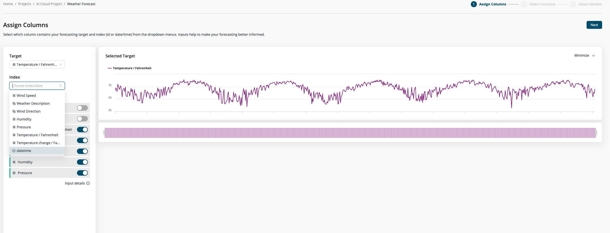
Step 1: Choose target and index columns

With Auto Forecasting it is very easy to build a forecasting model. In the first step you choose the column you want to predict -- the target column -- and an index column (if available). The index can be any date or numerical column, but it needs to include only unique values. If no index column is selected, the original order of the data used as a default.

In both cases you can inspect your selection as a line chart with the index column as x-axis and the target values as y-axis.

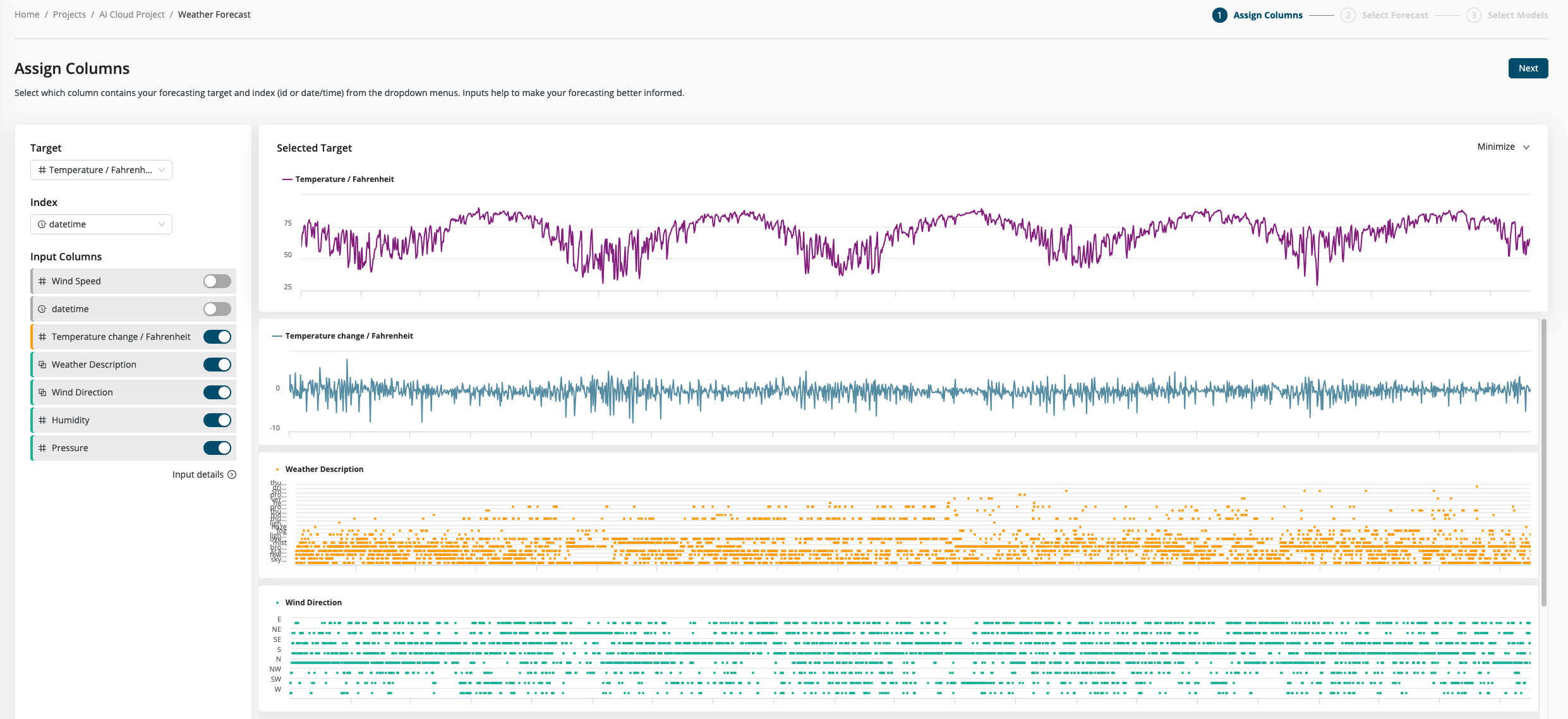
Step 2: Select inputs

Not all your data columns will help you make an accurate forecast. By discarding some of the columns, you may speed up your model-building and/or improve the model's performance. The input data is shown as line charts with the same x-axis as the target. You can use these charts to help you identify relevant columns for inclusion. With the toggle buttons you can select which columns to include.

Next to column names we show quality tags in green, yellow and red to help you identify good input candidates. By clicking on Input details, you can get additional information about the quality of the columns.

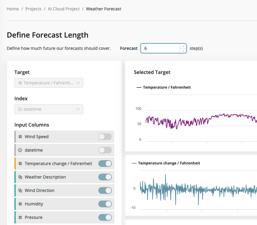
Step 3: Select forecast length

The important next step is to select how far into the future the model should predict. The number of steps is based on the selected index column. If it's daily data, then one step will be one day, if it's hourly data then one hour and so on. The ideal forecast length depends on your actual use case. Sometimes having a good prediction for the next day is very valuable, sometimes a more long-term forecast is needed. The range the forecast model looks ahead is called its horizon.

The trade-off here is that a shorter forecast horizon might return a more accurate model, while a longer horizon increases the uncertainty and the model complexity. If your data has very small steps in the index columns, but you want a longer forecast, it makes sense to aggregate the data first to get a better representation.

For example, your weather station records a new data point every minute. For a forecast of the next day, it makes sense to aggregate that data first to hourly or even daily averages.

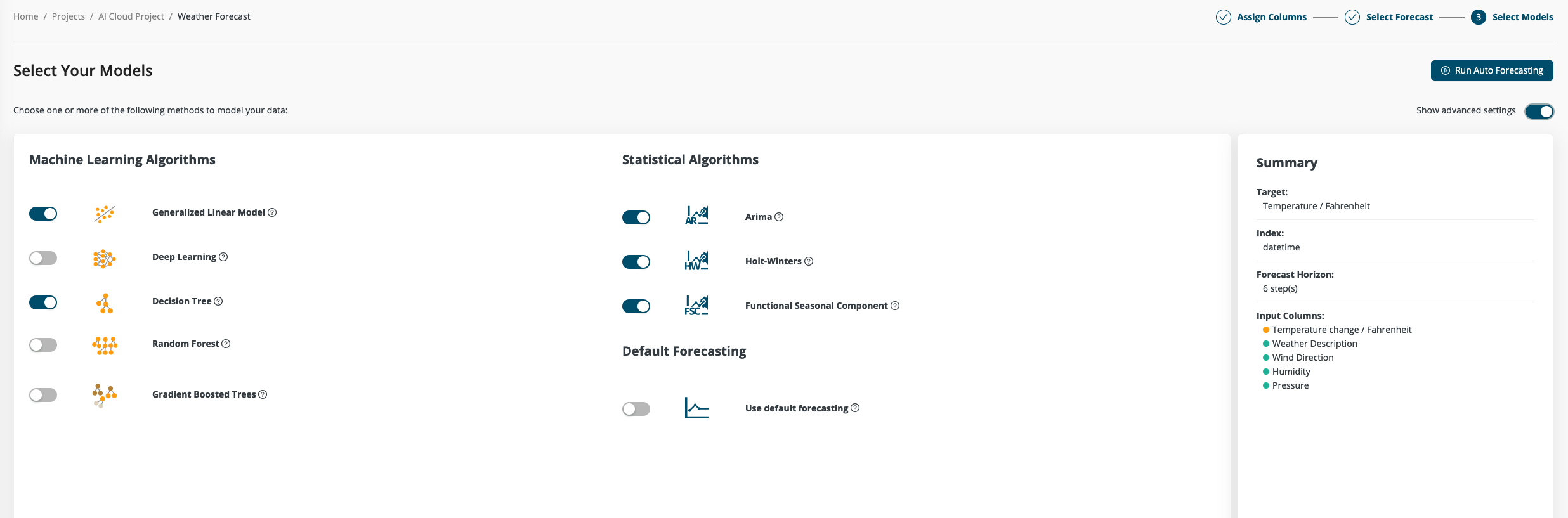
Step 4: Model selection

Auto Forecasting provides a selection of different algorithms to choose from. There are two different groups to choose from: machine learning algorithms and statistical algorithms.

Machine Learning Algorithms

In this group fall the same algorithms as used in a regular regression use case. They take and create predictions models for each step of the forecast horizon. The big advantage of this approach is that the algorithm can use multiple columns as additional source of information for the forecast and the different models can play out their different strengths. For additional information about the different models, you can check out the Auto Machine Learning documentation.

Statistical Algorithms

Statistical algorithms take a different approach for creating a forecast. Instead of taking a fixed look back, they try to learn and simulate the behavior of the target column. They analyze the values for trends and repeating patterns and build a statistical model to predict the most likely next values in the series.

From a practical standpoint, the biggest difference is that these algorithms only take the original series as input. That's why they are also often called univariate models, as there is only one variable. While this seems like a strong restriction compared to the machine learning approach, those algorithms are a stable and proven tool in the forecasting business. Their biggest strength lies in detecting long-running trends and seasonal or repeating patterns in the data. Because in nearly all real-world time series data, there is a strong repeating effect that regularly occurs. Examples are seasonal or monthly effects, weekdays, or daily patterns. If there's such a pattern in your data -- and they are often very easy to spot in the charts -- then statistical algorithms are very strong contenders to machine learning algorithms on finding them and incorporating them into the forecast. Also, they tend to run fast and to return results quickly.

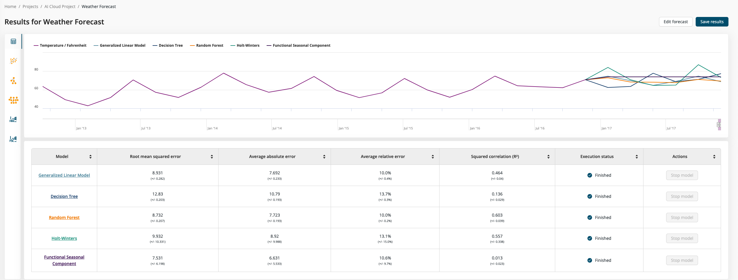
Step 5: Inspect results

Once all models have completed their training, you can see the different forecast results in a combined chart. The main line represents the initial data. The forecast values for each algorithm are directly attached to the original data and continue to the right up to the selected horizon.

Below the visual representation is a table that lists different performance metrics for each model. The performance measures are calculated by running a so-called sliding window validation. This method takes a subset of the data and runs the forecast model on it. The predicted values are then compared to the actual values that come next after the current window. This training and test window set is moved over the original data to calculate the average performance values.

The training windows can be inspected in detail for each algorithm on a separate details page. From that page, the final steps are either to store the forecast results as a new data set or open the workflow that was used to build the forecast. With this workflow in hand, it's easy to either fine tune the model on your own or create a deployment to forecast new values over time.